Single trap#
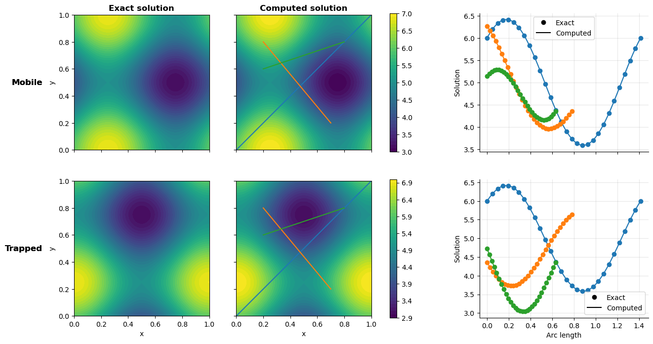
The MMS case verifies the implementation of trapping in FESTIM. Only one trap is considered for simplicity, but the same principle applies for more traps. Exact solutions are defined for both the mobile concentration and the trapped concentration.
(18)#\[\begin{align}
c_\mathrm{m, exact} &= 5 + \sin{\left(2 \pi x \right)} + \cos{\left(2 \pi y \right)} \\
c_\mathrm{t, exact} &= 5 + \cos{\left(2 \pi x \right)} + \sin{\left(2 \pi y \right)}
\end{align}\]
The trap density is \(n = 2 \ c_\mathrm{t,exact} \), the trapping rate is \(k = 0.1\), the detrapping rate is \(p = 0.2\), and the diffusivity is \(D=5\). MMS sources are obtained for both the mobile concentration and the trapped concentration:
(19)#\[\begin{align}
S_\mathrm{m} &= -D \nabla^2 c_\mathrm{m, exact} + k c_\mathrm{m, exact} (n - c_\mathrm{t, exact}) - p c_\mathrm{t, exact} \\
S_\mathrm{t} &= - k c_\mathrm{m, exact} (n - c_\mathrm{t, exact}) + p c_\mathrm{t, exact}
\end{align}\]
Again, the computed solution agrees very well with the exact solution.
FESTIM code#
Show code cell source
import festim as F
import sympy as sp
import fenics as f
import matplotlib as mpl
import matplotlib.pyplot as plt
import numpy as np

# Create and mark the mesh

fenics_mesh = f.UnitSquareMesh(100, 100)

left_surface = f.CompiledSubDomain("near(x[0], 0.0)")
right_surface = f.CompiledSubDomain("near(x[0], 1.0)")
top_surface = f.CompiledSubDomain("near(x[1], 1.0)")
bottom_surface = f.CompiledSubDomain("near(x[1], 0.0)")

volume_markers = f.MeshFunction("size_t", fenics_mesh, fenics_mesh.topology().dim())
volume_markers.set_all(1)

surface_markers = f.MeshFunction(
    "size_t", fenics_mesh, fenics_mesh.topology().dim() - 1
)
surface_markers.set_all(0)
left_surface.mark(surface_markers, 1)
top_surface.mark(surface_markers, 2)
right_surface.mark(surface_markers, 3)
bottom_surface.mark(surface_markers, 4)

# Create the FESTIM model
my_model = F.Simulation()

my_model.mesh = F.Mesh(
    fenics_mesh, volume_markers=volume_markers, surface_markers=surface_markers
)

# Variational formulation
x = F.x
y = F.y

exact_solution_mobile = (
    5 + sp.sin(2 * sp.pi * (x)) + sp.cos(2 * sp.pi * y)
)  # exact solution
exact_solution_trapped = (
    5 + sp.cos(2 * sp.pi * (x)) + sp.sin(2 * sp.pi * y)
)  # exact solution


def grad(u):
    """Computes the gradient of a function u.

    Args:
        u (sympy.Expr): a sympy function

    Returns:
        sympy.Matrix: the gradient of u
    """
    return sp.Matrix([sp.diff(u, x), sp.diff(u, y)])


def div(u):
    """Computes the divergence of a vector field u.

    Args:
        u (sympy.Matrix): a sympy vector field

    Returns:
        sympy.Expr: the divergence of u
    """
    return sp.diff(u[0], x) + sp.diff(u[1], y)


my_model.T = F.Temperature(value=500)

my_mat = F.Material(id=1, D_0=5, E_D=0)
my_model.materials = my_mat

density = 2 * exact_solution_trapped
my_trap = F.Trap(
    id=1,
    k_0=0.1,
    E_k=0,
    p_0=0.2,
    E_p=0,
    density=density,
    materials=my_model.materials.materials[0],
)
my_model.traps = [my_trap]


# source term left
k = my_trap.k_0 * sp.exp(-my_trap.E_k / my_model.T.value)
p = my_trap.p_0 * sp.exp(-my_trap.E_p / my_model.T.value)
D = my_mat.D_0 * sp.exp(-my_mat.E_D / my_model.T.value)

f_mobile = (
    -div(D * grad(exact_solution_mobile))
    + k * exact_solution_mobile * (density - exact_solution_trapped)
    - p * exact_solution_trapped
)
f_trap = (
    -k * exact_solution_mobile * (density - exact_solution_trapped)
    + p * exact_solution_trapped
)

print(
    f"Source term left: {sp.latex(f_mobile.simplify().subs('x[0]', 'x').subs('x[1]', 'y'))}"
)
print(
    f"Source term right: {sp.latex(f_trap.simplify().subs('x[0]', 'x').subs('x[1]', 'y'))}"
)

my_model.sources = [
    F.Source(f_mobile, volume=1, field="0"),
    F.Source(f_trap, volume=1, field="1"),
]

my_model.boundary_conditions = [
    F.DirichletBC(surfaces=[1, 2, 3, 4], value=exact_solution_mobile, field="solute"),
    F.DirichletBC(surfaces=[1, 2, 3, 4], value=exact_solution_trapped, field=1),
]

my_model.settings = F.Settings(
    absolute_tolerance=1e-10,
    relative_tolerance=1e-10,
    transient=False,
)

my_model.initialise()
my_model.run()
Show code cell output
/home/docs/checkouts/readthedocs.org/user_builds/festim-vv-report/conda/v1.0/lib/python3.11/site-packages/festim/materials/materials.py:34: DeprecationWarning: The materials attribute will be deprecated in a future release, please use festim.Materials as a list instead
  warnings.warn(
Source term left: \left(0.1 \sin{\left(2 \pi x \right)} + 0.1 \cos{\left(2 \pi y \right)} + 0.5\right) \left(\sin{\left(2 \pi y \right)} + \cos{\left(2 \pi x \right)} + 5\right) + 20 \pi^{2} \sin{\left(2 \pi x \right)} - 0.2 \sin{\left(2 \pi y \right)} - 0.2 \cos{\left(2 \pi x \right)} + 20 \pi^{2} \cos{\left(2 \pi y \right)} - 1.0
Source term right: - \left(0.1 \sin{\left(2 \pi x \right)} + 0.1 \cos{\left(2 \pi y \right)} + 0.5\right) \left(\sin{\left(2 \pi y \right)} + \cos{\left(2 \pi x \right)} + 5\right) + 0.2 \sin{\left(2 \pi y \right)} + 0.2 \cos{\left(2 \pi x \right)} + 1.0
Calling FFC just-in-time (JIT) compiler, this may take some time.
Defining initial values
Defining variational problem
Defining source terms
Defining boundary conditions
Solving steady state problem...
Calling FFC just-in-time (JIT) compiler, this may take some time.
Calling FFC just-in-time (JIT) compiler, this may take some time.
Calling FFC just-in-time (JIT) compiler, this may take some time.
Solved problem in 2.80 s
Comparison with exact solution#
Show code cell source
# export exact solution

exact_solution_mobile = f.Expression(sp.printing.ccode(exact_solution_mobile), degree=2)
exact_solution_trapped = f.Expression(
    sp.printing.ccode(exact_solution_trapped), degree=2
)
V = f.FunctionSpace(my_model.mesh.mesh, "CG", 1)
exact_solution_mobile = f.project(exact_solution_mobile, V)
exact_solution_trapped = f.project(exact_solution_trapped, V)

computed_solution_mobile = my_model.h_transport_problem.mobile.post_processing_solution
E = f.errornorm(computed_solution_mobile, exact_solution_mobile, "L2")
print(f"L2 error mobile: {E:.2e}")

computed_solution_trap = my_trap.post_processing_solution
E = f.errornorm(computed_solution_trap, exact_solution_trapped, "L2")
print(f"L2 error trap: {E:.2e}")

# plot exact solution and computed solution
fig, (axs_top, axs_bot) = plt.subplots(2, 3, figsize=(15, 8), sharex="col")
plt.sca(axs_top[0])
plt.title("Exact solution", weight="bold")
CS1 = f.plot(exact_solution_mobile)
plt.sca(axs_top[1])
plt.title("Computed solution", weight="bold")
CS2 = f.plot(computed_solution_mobile)

plt.colorbar(CS2, ax=[axs_top[0], axs_top[1]], shrink=1)

plt.sca(axs_bot[0])
CS3 = f.plot(exact_solution_trapped)
plt.sca(axs_bot[1])
CS4 = f.plot(computed_solution_trap)

plt.colorbar(CS4, ax=[axs_bot[0], axs_bot[1]], shrink=1)

for CS in [CS1, CS2, CS3, CS4]:
    CS.set_edgecolor("face")

pad = 5  # in points
row_labels = ["Mobile", "Trapped"]
for ax, row in zip([axs_top[0], axs_bot[0]], row_labels):
    ax.annotate(
        row,
        xy=(0, 0.5),
        xytext=(-ax.yaxis.labelpad - pad, 0),
        xycoords=ax.yaxis.label,
        textcoords="offset points",
        size="large",
        ha="right",
        va="center",
        weight="bold",
    )
axs_top[0].set_ylabel("y")
axs_bot[0].set_ylabel("y")
axs_bot[0].set_xlabel("x")
axs_bot[1].set_xlabel("x")

axs_top[0].sharey(axs_top[1])
plt.setp(axs_top[1].get_yticklabels(), visible=False)
axs_bot[0].sharey(axs_bot[1])
plt.setp(axs_bot[1].get_yticklabels(), visible=False)


def compute_arc_length(xs, ys):
    """Computes the arc length of x,y points based
    on x and y arrays
    """
    points = np.vstack((xs, ys)).T
    distance = np.linalg.norm(points[1:] - points[:-1], axis=1)
    arc_length = np.insert(np.cumsum(distance), 0, [0.0])
    return arc_length


# define the profiles
profiles = [
    {"start": (0.0, 0.0), "end": (1.0, 1.0)},
    {"start": (0.2, 0.8), "end": (0.7, 0.2)},
    {"start": (0.2, 0.6), "end": (0.8, 0.8)},
]

# plot the exact solution and the profile lines on the left subplot
for axs, exact, computed in zip(
    [axs_top, axs_bot],
    [exact_solution_mobile, exact_solution_trapped],
    [
        computed_solution_mobile,
        computed_solution_trap,
    ],
):
    # plot the profiles on the right subplot
    for i, profile in enumerate(profiles):
        start_x, start_y = profile["start"]
        end_x, end_y = profile["end"]
        plt.sca(axs[1])
        (l,) = plt.plot([start_x, end_x], [start_y, end_y])

        plt.sca(axs[2])

        points_x_exact = np.linspace(start_x, end_x, num=30)
        points_y_exact = np.linspace(start_y, end_y, num=30)
        arc_length_exact = compute_arc_length(points_x_exact, points_y_exact)
        u_values = [exact(x, y) for x, y in zip(points_x_exact, points_y_exact)]

        points_x = np.linspace(start_x, end_x, num=100)
        points_y = np.linspace(start_y, end_y, num=100)
        arc_lengths = compute_arc_length(points_x, points_y)
        computed_values = [computed(x, y) for x, y in zip(points_x, points_y)]

        (exact_line,) = plt.plot(
            arc_length_exact,
            u_values,
            color=l.get_color(),
            marker="o",
            linestyle="None",
        )
        (computed_line,) = plt.plot(arc_lengths, computed_values, color=l.get_color())

    plt.sca(axs[2])
    plt.ylabel("Solution")

    legend_marker = mpl.lines.Line2D(
        [],
        [],
        color="black",
        marker=exact_line.get_marker(),
        linestyle="None",
        label="Exact",
    )
    legend_line = mpl.lines.Line2D([], [], color="black", label="Computed")
    plt.legend(
        [legend_marker, legend_line],
        [legend_marker.get_label(), legend_line.get_label()],
    )

    plt.grid(alpha=0.3)
    plt.gca().spines[["right", "top"]].set_visible(False)

axs_bot[-1].set_xlabel("Arc length")

pad = 5  # in points
row_labels = ["Mobile", "Trapped"]
for ax, row in zip([axs_top[0], axs_bot[0]], row_labels):
    ax.annotate(
        row,
        xy=(0, 0.5),
        xytext=(-ax.yaxis.labelpad - pad, 0),
        xycoords=ax.yaxis.label,
        textcoords="offset points",
        size="large",
        ha="right",
        va="center",
        weight="bold",
    )

plt.show()
L2 error mobile: 3.29e-04
L2 error trap: 2.57e-04