Simple diffusion with varying temperature#
This is an extension of the simple MMS example with a non-homogenous temperature gradient.
We will only consider diffusion of hydrogen in a unit square domain \(\Omega\) at steady state with an homogeneous diffusion coefficient \(D\).
We will assume a temperature gradient of \(T = 300 + x\) over the domain \(\Omega\) so the diffusivity coefficient \(D = D_0 \exp\left[-\frac{E_D}{k_B T}\right]\).
Moreover, a Dirichlet boundary condition will be assumed on the boundaries \(\partial \Omega \).
The problem is therefore:
The exact solution for mobile concentration is:
Injecting (9) in (8), we obtain the expressions of \(S\) and \(c_0\):
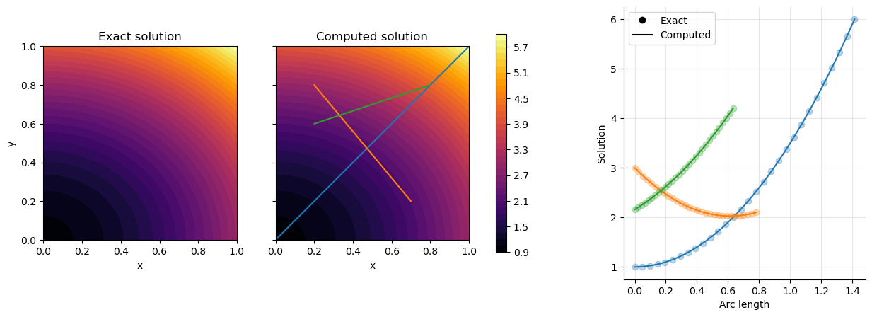
We can then run a FESTIM model with these values and compare the numerical solution with \(c_\mathrm{exact}\).
FESTIM code#
Show code cell content
import festim as F
import sympy as sp
import fenics as f
import matplotlib as mpl
import matplotlib.pyplot as plt
import numpy as np
import sympy as sp

# Create and mark the mesh
nx = ny = 100
fenics_mesh = f.UnitSquareMesh(nx, ny)


volume_markers = f.MeshFunction("size_t", fenics_mesh, fenics_mesh.topology().dim())
volume_markers.set_all(1)

surface_markers = f.MeshFunction(
    "size_t", fenics_mesh, fenics_mesh.topology().dim() - 1
)
surface_markers.set_all(0)

class Boundary(f.SubDomain):
    def inside(self, x, on_boundary):
        return on_boundary

boundary = Boundary()
boundary.mark(surface_markers, 1)
# Create the FESTIM model
my_model = F.Simulation()

my_model.mesh = F.Mesh(
    fenics_mesh, volume_markers=volume_markers, surface_markers=surface_markers
)

# Variational formulation
exact_solution = (
    1 + 2 * F.x**2 + 3 * F.y**2
)  # exact solution

T = 300 + F.x

D_0 = 2
E_D = 2
D = D_0 * sp.exp(-E_D / (F.k_B * T))
S = - D * (4 * F.x * E_D/(F.k_B * T**2) + 10)

my_model.sources = [
    F.Source(S, volume=1, field="solute"),
]

my_model.boundary_conditions = [
    F.DirichletBC(surfaces=[1], value=exact_solution, field="solute"),
]

my_model.materials = F.Material(id=1, D_0=D_0, E_D=E_D)

my_model.T = F.Temperature(T)

my_model.settings = F.Settings(
    absolute_tolerance=1e-10,
    relative_tolerance=1e-10,
    transient=False,
)

my_model.initialise()
my_model.run()
Defining initial values
Defining variational problem
Defining source terms
Defining boundary conditions
Solving steady state problem...
Calling FFC just-in-time (JIT) compiler, this may take some time.
Calling FFC just-in-time (JIT) compiler, this may take some time.
Solved problem in 1.50 s
Comparison with exact solution#
Show code cell source
c_exact = f.Expression(sp.printing.ccode(exact_solution), degree=4)
c_exact = f.project(c_exact, f.FunctionSpace(my_model.mesh.mesh, "CG", 1))

computed_solution = my_model.h_transport_problem.mobile.post_processing_solution
E = f.errornorm(computed_solution, c_exact, "L2")
print(f"L2 error: {E:.2e}")

# plot exact solution and computed solution
fig, axs = plt.subplots(1, 3, figsize=(15, 5))
plt.sca(axs[0])
plt.title("Exact solution")
plt.xlabel("x")
plt.ylabel("y")
CS1 = f.plot(c_exact, cmap="inferno")
plt.sca(axs[1])
plt.xlabel("x")
plt.title("Computed solution")
CS2 = f.plot(computed_solution, cmap="inferno")

plt.colorbar(CS2, ax=[axs[0], axs[1]], shrink=0.8)

axs[0].sharey(axs[1])
plt.setp(axs[1].get_yticklabels(), visible=False)

for CS in [CS1, CS2]:
    CS.set_edgecolor("face")


def compute_arc_length(xs, ys):
    """Computes the arc length of x,y points based
    on x and y arrays
    """
    points = np.vstack((xs, ys)).T
    distance = np.linalg.norm(points[1:] - points[:-1], axis=1)
    arc_length = np.insert(np.cumsum(distance), 0, [0.0])
    return arc_length


# define the profiles
profiles = [
    {"start": (0.0, 0.0), "end": (1.0, 1.0)},
    {"start": (0.2, 0.8), "end": (0.7, 0.2)},
    {"start": (0.2, 0.6), "end": (0.8, 0.8)},
]

# plot the profiles on the right subplot
for i, profile in enumerate(profiles):
    start_x, start_y = profile["start"]
    end_x, end_y = profile["end"]
    plt.sca(axs[1])
    (l,) = plt.plot([start_x, end_x], [start_y, end_y])

    plt.sca(axs[2])

    points_x_exact = np.linspace(start_x, end_x, num=30)
    points_y_exact = np.linspace(start_y, end_y, num=30)
    arc_length_exact = compute_arc_length(points_x_exact, points_y_exact)
    u_values = [c_exact(x, y) for x, y in zip(points_x_exact, points_y_exact)]

    points_x = np.linspace(start_x, end_x, num=100)
    points_y = np.linspace(start_y, end_y, num=100)
    arc_lengths = compute_arc_length(points_x, points_y)
    computed_values = [computed_solution(x, y) for x, y in zip(points_x, points_y)]

    (exact_line,) = plt.plot(
        arc_length_exact, u_values, color=l.get_color(), marker="o", linestyle="None", alpha=0.3
    )
    (computed_line,) = plt.plot(arc_lengths, computed_values, color=l.get_color())

plt.sca(axs[2])
plt.xlabel("Arc length")
plt.ylabel("Solution")

legend_marker = mpl.lines.Line2D(
    [],
    [],
    color="black",
    marker=exact_line.get_marker(),
    linestyle="None",
    label="Exact",
)
legend_line = mpl.lines.Line2D([], [], color="black", label="Computed")
plt.legend(
    [legend_marker, legend_line], [legend_marker.get_label(), legend_line.get_label()]
)

plt.grid(alpha=0.3)
plt.gca().spines[["right", "top"]].set_visible(False)
plt.show()
L2 error: 8.33e-05
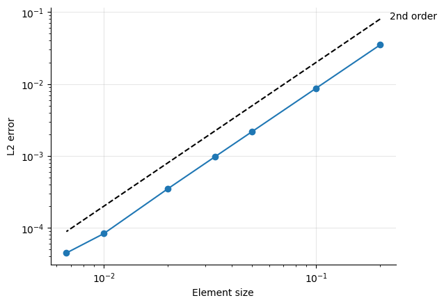
Compute convergence rates#
It is also possible to compute how the numerical error decreases as we increase the number of cells. By iteratively refining the mesh, we find that the error exhibits a second order convergence rate. This is expected for this particular problem as first order finite elements are used.
Show code cell content
errors = []
ns = [5, 10, 20, 30, 50, 100, 150]

for n in ns:
    nx = ny = n
    fenics_mesh = f.UnitSquareMesh(nx, ny)

    volume_markers = f.MeshFunction("size_t", fenics_mesh, fenics_mesh.topology().dim())
    volume_markers.set_all(1)

    surface_markers = f.MeshFunction(
        "size_t", fenics_mesh, fenics_mesh.topology().dim() - 1
    )
    surface_markers.set_all(0)

    class Boundary(f.SubDomain):
        def inside(self, x, on_boundary):
            return on_boundary

    boundary = Boundary()
    boundary.mark(surface_markers, 1)

    my_model.mesh = F.Mesh(
        fenics_mesh, volume_markers=volume_markers, surface_markers=surface_markers
    )

    my_model.initialise()
    my_model.run()

    computed_solution = my_model.h_transport_problem.mobile.post_processing_solution
    errors.append(f.errornorm(computed_solution, c_exact, "L2"))
Defining initial values
Defining variational problem
Defining source terms
Defining boundary conditions
Solving steady state problem...
Solved problem in 0.00 s
Defining initial values
Defining variational problem
Defining source terms
Defining boundary conditions
Solving steady state problem...
Solved problem in 0.00 s
Defining initial values
Defining variational problem
Defining source terms
Defining boundary conditions
Solving steady state problem...
Solved problem in 0.00 s
Defining initial values
Defining variational problem
Defining source terms
Defining boundary conditions
Solving steady state problem...
Solved problem in 0.00 s
Defining initial values
Defining variational problem
Defining source terms
Defining boundary conditions
Solving steady state problem...
Solved problem in 0.00 s
Defining initial values
Defining variational problem
Defining source terms
Defining boundary conditions
Solving steady state problem...
Solved problem in 0.10 s
Defining initial values
Defining variational problem
Defining source terms
Defining boundary conditions
Solving steady state problem...
Solved problem in 0.30 s
Show code cell source
h = 1 / np.array(ns)

plt.loglog(h, errors, marker="o")
plt.xlabel("Element size")
plt.ylabel("L2 error")

plt.loglog(h, 2 * h**2, linestyle="--", color="black")
plt.annotate("2nd order", (h[0], 2 * h[0]**2), textcoords="offset points", xytext=(10, 0))

plt.grid(alpha=0.3)
plt.gca().spines[["right", "top"]].set_visible(False)