Heat transfer multi-material#
This case verifies the implementation of the heat transfer solver in FESTIM. Two materials with different thermal conductivities are defined: \(\lambda_\mathrm{left} = 2\) and \(\lambda_\mathrm{right} = 5\).
(13)#\[\begin{split}
\begin{align}
&\nabla \cdot (\lambda \nabla T) + Q = 0 \quad \text{on } \Omega \\
& T = T_0 \quad \text{on } \partial\Omega
\end{align}
\end{split}\]
The exact solution for temperature is:
(14)#\[
\begin{equation}
T_\mathrm{exact} = 1 + \sin{\left(\pi \left(2 x + 0.5\right) \right)} + \cos{\left(2 \pi y \right)}
\end{equation}
\]
The manufactured solution is chosen so that the thermal flux \(-\lambda \nabla T \cdot \textbf{n}\) is continuous across the interface.
By injecting (14) in (13) we can obtain:
(15)#\[\begin{align}
Q_\mathrm{left} &= 8 \pi^{2} \left(\cos{\left(2 \pi x \right)} + \cos{\left(2 \pi y \right)}\right) \\
Q_\mathrm{right} &= 20 \pi^{2} \left(\cos{\left(2 \pi x \right)} + \cos{\left(2 \pi y \right)}\right) \\
T_0 &= T_\mathrm{exact}
\end{align}\]
FESTIM code#
Show code cell source
import festim as F
import sympy as sp
import fenics as f
import matplotlib as mpl
import matplotlib.pyplot as plt
import numpy as np

# Create and mark the mesh

fenics_mesh = f.UnitSquareMesh(100, 100)

left_surface = f.CompiledSubDomain("near(x[0], 0.0)")
right_surface = f.CompiledSubDomain("near(x[0], 1.0)")
top_right_surface = f.CompiledSubDomain("near(x[1], 1.0) && x[0] > 0.5")
top_left_surface = f.CompiledSubDomain("near(x[1], 1.0) && x[0] < 0.5")
bottom_right_surface = f.CompiledSubDomain("near(x[1], 0.0) && x[0] > 0.5")
bottom_left_surface = f.CompiledSubDomain("near(x[1], 0.0) && x[0] < 0.5")


class LeftSubdomain(f.SubDomain):
    def inside(self, x, on_boundary):
        return f.between(x[0], (0.0, 0.5))


class RightSubdomain(f.SubDomain):
    def inside(self, x, on_boundary):
        return f.between(x[0], (0.5, 1.0))


volume_markers = f.MeshFunction("size_t", fenics_mesh, fenics_mesh.topology().dim())
volume_markers.set_all(0)
left_volume = LeftSubdomain()
right_volume = RightSubdomain()

left_volume.mark(volume_markers, 1)
right_volume.mark(volume_markers, 2)

surface_markers = f.MeshFunction(
    "size_t", fenics_mesh, fenics_mesh.topology().dim() - 1
)
surface_markers.set_all(0)
left_surface.mark(surface_markers, 1)
top_left_surface.mark(surface_markers, 2)
top_right_surface.mark(surface_markers, 3)
right_surface.mark(surface_markers, 4)
bottom_right_surface.mark(surface_markers, 5)
bottom_left_surface.mark(surface_markers, 6)

# Create the FESTIM model
my_model = F.Simulation()

my_model.mesh = F.Mesh(
    fenics_mesh, volume_markers=volume_markers, surface_markers=surface_markers
)

# Variational formulation
x = F.x
y = F.y

exact_solution = (
    1 + sp.sin(2 * sp.pi * (x + 0.25)) + sp.cos(2 * sp.pi * y)
)  # exact solution

lambda_left, lambda_right = 2, 5  # diffusion coeffs


def grad(u):
    """Computes the gradient of a function u.

    Args:
        u (sympy.Expr): a sympy function

    Returns:
        sympy.Matrix: the gradient of u
    """
    return sp.Matrix([sp.diff(u, x), sp.diff(u, y)])


def div(u):
    """Computes the divergence of a vector field u.

    Args:
        u (sympy.Matrix): a sympy vector field

    Returns:
        sympy.Expr: the divergence of u
    """
    return sp.diff(u[0], x) + sp.diff(u[1], y)


# source term left
source_left = -div(lambda_left * grad(exact_solution))
source_right = -div(lambda_right * grad(exact_solution))

print(
    f"Source term left: {sp.latex(source_left.simplify().subs('x[0]', 'x').subs('x[1]', 'y'))}"
)
print(
    f"Source term right: {sp.latex(source_right.simplify().subs('x[0]', 'x').subs('x[1]', 'y'))}"
)

my_model.sources = [
    F.Source(source_left, volume=1, field="T"),
    F.Source(source_right, volume=2, field="T"),
]

my_model.boundary_conditions = [
    F.DirichletBC(surfaces=[1, 2, 6], value=exact_solution, field="T"),
    F.DirichletBC(surfaces=[3, 4, 5], value=exact_solution, field="T"),
]

left_material = F.Material(id=1, D_0=1, E_D=0, thermal_cond=lambda_left)
right_material = F.Material(id=2, D_0=1, E_D=0, thermal_cond=lambda_right)

my_model.materials = [left_material, right_material]

my_model.T = F.HeatTransferProblem(transient=False)

my_model.exports = [F.XDMFExport("T")]

my_model.settings = F.Settings(
    absolute_tolerance=1e-10,
    relative_tolerance=1e-10,
    transient=False,
)

my_model.initialise()
my_model.run()
Show code cell output
Source term left: 8 \pi^{2} \left(\cos{\left(2 \pi x \right)} + \cos{\left(2 \pi y \right)}\right)
Source term right: 20 \pi^{2} \left(\cos{\left(2 \pi x \right)} + \cos{\left(2 \pi y \right)}\right)
Defining variational problem heat transfers
Solving stationary heat equation
Calling FFC just-in-time (JIT) compiler, this may take some time.
Calling FFC just-in-time (JIT) compiler, this may take some time.
Defining initial values
Defining variational problem
Defining source terms
Defining boundary conditions
Solving steady state problem...
Calling FFC just-in-time (JIT) compiler, this may take some time.
Calling FFC just-in-time (JIT) compiler, this may take some time.
Solved problem in 1.10 s
Comparison with exact solution#
Show code cell source
T_exact = f.Expression(sp.printing.ccode(exact_solution), degree=2)
T_exact = f.project(T_exact, f.FunctionSpace(my_model.mesh.mesh, "CG", 1))

computed_solution = my_model.T.T
E = f.errornorm(computed_solution, T_exact, "L2")
print(f"L2 error: {E:.2e}")

# plot exact solution and computed solution
fig, axs = plt.subplots(1, 3, figsize=(15, 5))
plt.sca(axs[0])
plt.title("Exact solution")
plt.xlabel("x")
plt.ylabel("y")
CS1 = f.plot(T_exact, cmap="inferno")
plt.sca(axs[1])
plt.xlabel("x")
plt.title("Computed solution")
CS2 = f.plot(computed_solution, cmap="inferno")

plt.colorbar(CS2, ax=[axs[0], axs[1]], shrink=0.8)

axs[0].sharey(axs[1])
plt.setp(axs[1].get_yticklabels(), visible=False)

for CS in [CS1, CS2]:
    CS.set_edgecolor("face")


def compute_arc_length(xs, ys):
    """Computes the arc length of x,y points based
    on x and y arrays
    """
    points = np.vstack((xs, ys)).T
    distance = np.linalg.norm(points[1:] - points[:-1], axis=1)
    arc_length = np.insert(np.cumsum(distance), 0, [0.0])
    return arc_length


# define the profiles
profiles = [
    {"start": (0.0, 0.0), "end": (1.0, 1.0)},
    {"start": (0.2, 0.8), "end": (0.7, 0.2)},
    {"start": (0.2, 0.6), "end": (0.8, 0.8)},
]

# plot the profiles on the right subplot
for i, profile in enumerate(profiles):
    start_x, start_y = profile["start"]
    end_x, end_y = profile["end"]
    plt.sca(axs[1])
    (l,) = plt.plot([start_x, end_x], [start_y, end_y])

    plt.sca(axs[2])

    points_x_exact = np.linspace(start_x, end_x, num=30)
    points_y_exact = np.linspace(start_y, end_y, num=30)
    arc_length_exact = compute_arc_length(points_x_exact, points_y_exact)
    u_values = [T_exact(x, y) for x, y in zip(points_x_exact, points_y_exact)]

    points_x = np.linspace(start_x, end_x, num=100)
    points_y = np.linspace(start_y, end_y, num=100)
    arc_lengths = compute_arc_length(points_x, points_y)
    computed_values = [computed_solution(x, y) for x, y in zip(points_x, points_y)]

    (exact_line,) = plt.plot(
        arc_length_exact, u_values, color=l.get_color(), marker="o", linestyle="None"
    )
    (computed_line,) = plt.plot(arc_lengths, computed_values, color=l.get_color())

plt.sca(axs[2])
plt.xlabel("Arc length")
plt.ylabel("Solution")

legend_marker = mpl.lines.Line2D(
    [],
    [],
    color="black",
    marker=exact_line.get_marker(),
    linestyle="None",
    label="Exact",
)
legend_line = mpl.lines.Line2D([], [], color="black", label="Computed")
plt.legend(
    [legend_marker, legend_line], [legend_marker.get_label(), legend_line.get_label()]
)

plt.grid(alpha=0.3)
plt.gca().spines[["right", "top"]].set_visible(False)
plt.show()
Calling FFC just-in-time (JIT) compiler, this may take some time.
L2 error: 3.31e-04
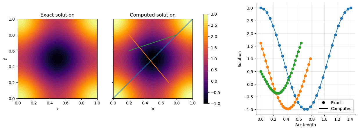
The computed solution and the exact solutions are in very good agreement.