Simple transient diffusion case

🏷 Tags: 2D MMS transient

This is a simple transient MMS example. We will only consider diffusion of hydrogen in a unit square domain \(\Omega\) at steady state with an homogeneous diffusion coefficient \(D\). Moreover, a Dirichlet boundary condition will be assumed on the boundaries \(\partial \Omega \).

The problem is therefore:

(5)\[\begin{split} \begin{align} &\nabla \cdot (D \ \nabla{c}) - \frac{\partial c}{\partial t} = -S \quad \text{on } \Omega ; \ t\geq 0 \\ & c = c_0 \quad \text{on } \partial \Omega ; \ t\geq 0 \\ & c = c_\mathrm{initial} \quad \text{on } \partial \Omega ; \ \text{at } t=0 \end{align} \end{split}\]

The exact solution for mobile concentration is:

(6)\[ \begin{equation} c_\mathrm{exact} = 1 + 2 x^2 + 3 y^2 t + 2t \end{equation} \]

Note

We use a manufactured solution that varies linearly with time (\(t^1\)), as the backward Euler scheme provides an exact solution in this case.

Injecting (6) in (5), we obtain the expressions of \(S\), \(c_0\), and \(c_\mathrm{initial}\):

(7)\[\begin{align} & S = 2 + 3 y^2 - (4 + 6t) D \\ & c_0 = c_\mathrm{exact} \\ & c_\mathrm{initial} = c_\mathrm{exact}(t=0) \end{align}\]

We can then run a FESTIM model with these values and compare the numerical solution with \(c_\mathrm{exact}\).

FESTIM code

Show code cell content

Hide code cell content

import festim as F
from mpi4py import MPI
import dolfinx
import numpy as np

# --- Create and mark the mesh ---
nx = ny = 100
fenics_mesh = dolfinx.mesh.create_unit_square(MPI.COMM_WORLD, nx, ny)

# --- FESTIM model setup ---
my_model = F.HydrogenTransportProblem()
H = F.Species("H")
my_model.species = [H]
my_model.mesh = F.Mesh(fenics_mesh)

# --- materials ---
D = 2
material = F.Material(D_0=D, E_D=0)

# --- subdomains ---
volume = F.VolumeSubdomain(id=1, material=material)
boundary = F.SurfaceSubdomain(id=1)
my_model.subdomains = [volume, boundary]

# --- define the exact solution ---
exact_solution = lambda x,t:1 + 2 * x[0]**2 + 3 * t * x[1]**2 + 2 * t 

# --- define the sources and boundary conditions ---
my_model.sources = [(F.ParticleSource(value=lambda x, t: 2 + 3 * x[1]**2 - (4 + 6 * t) * D , volume = volume, species=H))]
my_model.boundary_conditions = [
    F.FixedConcentrationBC(subdomain=boundary, value=exact_solution, species=H),
]

my_model.temperature = 500  # ignored in this problem

# --- output control ---
xdmf_file_name = "simple_transient_mobile.xdmf"
vtx_file_name = "simple_transient_mobile.bp"
my_model.exports = [
    F.XDMFExport(field=H, filename=xdmf_file_name),
    F.VTXSpeciesExport(field=H, filename=vtx_file_name, checkpoint=True),
    F.VTXSpeciesExport(field=H, filename="out.bp", checkpoint=False)
]


# --- time stepping ---
final_time = 17
dt = F.Stepsize(initial_value=1)
my_model.settings = F.Settings(
    atol=1e-10,
    rtol=1e-10,
    final_time=final_time,
    stepsize=dt,
)

my_model.initialise()
my_model.run()

/home/docs/checkouts/readthedocs.org/user_builds/festim-vv-report/conda/festim-2/lib/python3.11/site-packages/festim/coupled_heat_hydrogen_problem.py:1: TqdmExperimentalWarning: Using `tqdm.autonotebook.tqdm` in notebook mode. Use `tqdm.tqdm` instead to force console mode (e.g. in jupyter console)
  import tqdm.autonotebook

Comparison with exact solution

Show code cell source

Hide code cell source

import pyvista
from dolfinx.plot import vtk_mesh
import adios4dolfinx
from mpi4py import MPI

"""
Post-process FESTIM v2/VTX (.bp) output in Python with PyVista.

- Reads selected timesteps from a VTX/ADIOS2 file using adios4dolfinx
- For each timestep, computes the corresponding analytic "exact" field
- Plots a grid of comparisons between simulation and exact solutions:
  1 row per time instant
  2 columns: left = simulation, right = exact
"""


pyvista.start_xvfb()
pyvista.set_jupyter_backend("html")

def read_computed_solution(time: float):
    """Load FEM function at a given time from a VTX/ADIOS2 file."""
    mesh = adios4dolfinx.read_mesh(vtx_file_name, comm=MPI.COMM_WORLD)
    V = dolfinx.fem.functionspace(mesh, ("Lagrange", 1))
    u_in = dolfinx.fem.Function(V)
    adios4dolfinx.read_function(vtx_file_name, u_in, time=time, name=H.name)
    return u_in


def get_u_grid(u: dolfinx.fem.Function, label: str):
    """Convert a FEM function to a PyVista UnstructuredGrid and attach nodal data."""
    u_topology, u_cell_types, u_geometry = vtk_mesh(u.function_space)
    u_grid = pyvista.UnstructuredGrid(u_topology, u_cell_types, u_geometry)
    u_grid.point_data[label] = u.x.array.real
    u_grid.set_active_scalars(label)
    return u_grid

timestamps = adios4dolfinx.read_timestamps(vtx_file_name, MPI.COMM_WORLD, function_name=H.name)

for t_val in timestamps[::6]:
    t_val = float(t_val)

    computed_solution = read_computed_solution(t_val)
    u_grid_mobile = get_u_grid(computed_solution, "c_simulation")

    exact_solution_function = dolfinx.fem.Function(computed_solution.function_space)
    exact_solution_function.interpolate(
        lambda X: 1 + 2 * X[0] ** 2 + 3 * t_val * X[1] ** 2 + 2 * t_val
    )
    u_grid_mobile_exact = get_u_grid(exact_solution_function, "c_exact")

    print(f"t={float(t_val):g}s, Simulation result (left) vs. Exact result (right)")
    u_plotter = pyvista.Plotter(shape=(1, 2))
    
    u_plotter.subplot(0, 0)
    u_plotter.add_title("simulation",font_size = 20, color = "black")
    u_plotter.set_background("white")
    u_plotter.add_mesh(u_grid_mobile)
    contours_sim = u_grid_mobile.contour(9)
    u_plotter.add_mesh(contours_sim, color="white")
    u_plotter.add_text("Simulation", font_size=18,color="black", position="upper_edge")
    u_plotter.view_xy()

    u_plotter.subplot(0, 1)
    u_plotter.set_background("white")
    u_plotter.add_mesh(u_grid_mobile_exact)
    contours_ex = u_grid_mobile_exact.contour(9)
    u_plotter.add_mesh(contours_ex, color="white")
    u_plotter.view_xy()
    u_plotter.add_text("Exact", font_size=18,color="black", position="upper_edge")
    

    if not pyvista.OFF_SCREEN:
        u_plotter.show()
    else:
        figure = u_plotter.screenshot("comparison.png")

/home/docs/checkouts/readthedocs.org/user_builds/festim-vv-report/conda/festim-2/lib/python3.11/site-packages/pyvista/plotting/utilities/xvfb.py:48: PyVistaDeprecationWarning: This function is deprecated and will be removed in future version of PyVista. Use vtk-osmesa instead.
  warnings.warn(

t=1s, Simulation result (left) vs. Exact result (right)

t=7s, Simulation result (left) vs. Exact result (right)

t=13s, Simulation result (left) vs. Exact result (right)

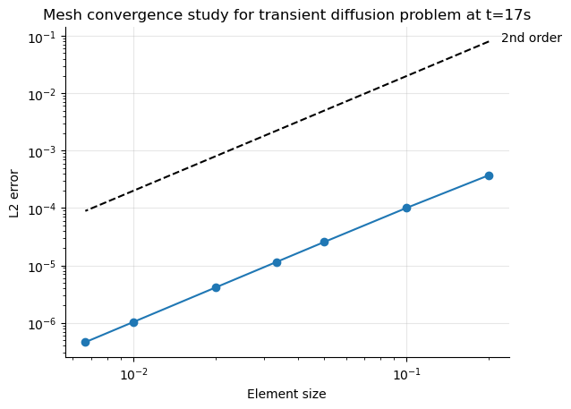
Compute convergence rates

It is also possible to compute how the numerical error decreases as we increase the number of cells. By iteratively refining the mesh, we find that the error exhibits a second order convergence rate. This is expected for this particular problem as first order finite elements are used.

Show code cell content

Hide code cell content

import matplotlib.pyplot as plt
import ufl
import dolfinx


def error_L2(u_computed, u_exact, degree_raise=3):
    # Create higher order function space
    degree = u_computed.function_space.ufl_element().degree
    family = u_computed.function_space.ufl_element().family_name
    mesh = u_computed.function_space.mesh
    W = dolfinx.fem.functionspace(mesh, (family, degree + degree_raise))

    # Interpolate exact solution, special handling if exact solution
    # is a ufl expression or a python lambda function
    u_ex_W = dolfinx.fem.Function(W)
    if isinstance(u_exact, ufl.core.expr.Expr):
        u_expr = dolfinx.fem.Expression(u_exact, W.element.interpolation_points)
        u_ex_W.interpolate(u_expr)
    else:
        u_ex_W.interpolate(u_exact)

    # Integrate the error
    error = dolfinx.fem.form(
        ufl.inner(u_computed - u_ex_W, u_computed - u_ex_W) * ufl.dx
    )
    error_local = dolfinx.fem.assemble_scalar(error)
    error_global = mesh.comm.allreduce(error_local, op=MPI.SUM)
    return np.sqrt(error_global)


errors = []
ns = [5, 10, 20, 30, 50, 100, 150]

for n in ns:
    nx = ny = n
    fenics_mesh = fenics_mesh = dolfinx.mesh.create_unit_square(MPI.COMM_WORLD, nx, ny)

    new_model = F.HydrogenTransportProblem()
    new_model.mesh = F.Mesh(fenics_mesh)

    new_model.species = my_model.species
    new_model.subdomains = my_model.subdomains
    new_model.sources = my_model.sources
    new_model.boundary_conditions = my_model.boundary_conditions
    new_model.temperature = my_model.temperature
    new_model.settings = my_model.settings

    new_model.initialise()
    new_model.run()
    
    # by default, get the last time step solution
    computed_solution = H.solution
    exact_solution_function = dolfinx.fem.Function(computed_solution.function_space)
    exact_solution_function.interpolate(
        lambda X: 1 + 2 * X[0] ** 2 + 3 * final_time * X[1] ** 2 + 2 * final_time
    )
    errors.append(error_L2(computed_solution, exact_solution_function))

h = 1 / np.array(ns)

plt.loglog(h, errors, marker="o")
plt.xlabel("Element size")
plt.ylabel("L2 error")
plt.title("Mesh convergence study for transient diffusion problem at t=17s")

plt.loglog(h, 2 * h**2, linestyle="--", color="black")
plt.annotate(
    "2nd order", (h[0], 2 * h[0] ** 2), textcoords="offset points", xytext=(10, 0)
)

plt.grid(alpha=0.3)
plt.gca().spines[["right", "top"]].set_visible(False)