Heat transfer multi-material#
This case verifies the implementation of the heat transfer solver in FESTIM. Two materials with different thermal conductivities are defined: \(\lambda_\mathrm{left} = 2\) and \(\lambda_\mathrm{right} = 5\).
(13)#\[\begin{split}
\begin{align}
&\nabla \cdot (\lambda \nabla T) + Q = 0 \quad \text{on } \Omega \\
& T = T_0 \quad \text{on } \partial\Omega
\end{align}
\end{split}\]
The exact solution for temperature is:
(14)#\[
\begin{equation}
T_\mathrm{exact} = 1 + \sin{\left(\pi \left(2 x + 0.5\right) \right)} + \cos{\left(2 \pi y \right)}
\end{equation}
\]
The manufactured solution is chosen so that the thermal flux \(-\lambda \nabla T \cdot \textbf{n}\) is continuous across the interface.
By injecting (14) in (13) we can obtain:
(15)#\[\begin{align}
Q_\mathrm{left} &= -\nabla \cdot (\lambda_\mathrm{left} \nabla T_\mathrm{exact}) \\
Q_\mathrm{right} &= -\nabla \cdot (\lambda_\mathrm{right} \nabla T_\mathrm{exact}) \\
T_0 &= T_\mathrm{exact}
\end{align}\]
FESTIM code#
import festim as F
import numpy as np

import dolfinx
import ufl
from mpi4py import MPI

nx = ny = 10
fenics_mesh = dolfinx.mesh.create_unit_square(MPI.COMM_WORLD, nx, ny)


class LeftSubdomain(F.VolumeSubdomain):
    def locate_subdomain_entities(self, mesh):
        return dolfinx.mesh.locate_entities(
            mesh, mesh.topology.dim, lambda x: x[0] < 0.5 + 1e-10
        )


class RightSubdomain(F.VolumeSubdomain):
    def locate_subdomain_entities(self, mesh):
        return dolfinx.mesh.locate_entities(
            mesh, mesh.topology.dim, lambda x: x[0] >= 0.5 - 1e-10
        )


boundary = F.SurfaceSubdomain(id=1)

# Create the FESTIM model
my_model = F.HeatTransferProblem()

my_model.mesh = F.Mesh(fenics_mesh)

lambda_left, lambda_right = 2, 5  # diffusion coeffs

mat_left = F.Material(D_0=1, E_D=0, thermal_conductivity=lambda_left)
mat_right = F.Material(D_0=1, E_D=0, thermal_conductivity=lambda_right)
left_volume = LeftSubdomain(id=1, material=mat_left)
right_volume = RightSubdomain(id=2, material=mat_right)

my_model.subdomains = [left_volume, right_volume, boundary]


def exact_solution(mod):
    return (
        lambda x: 1 + mod.sin(2 * mod.pi * (x[0] + 0.25)) + mod.cos(2 * mod.pi * x[1])
    )


exact_solution_ufl = exact_solution(ufl)

source_left = lambda x: -ufl.div(lambda_left * ufl.grad(exact_solution_ufl(x)))
source_right = lambda x: -ufl.div(lambda_right * ufl.grad(exact_solution_ufl(x)))

my_model.sources = [
    F.HeatSource(source_left, volume=left_volume),
    F.HeatSource(source_right, volume=right_volume),
]

my_model.boundary_conditions = [
    F.FixedTemperatureBC(subdomain=boundary, value=exact_solution_ufl),
]

my_model.settings = F.Settings(atol=1e-10, rtol=1e-10, transient=False)

my_model.initialise()
my_model.run()
Comparison with exact solution#
computed_solution = my_model.u

E_l2 = error_L2(computed_solution, exact_solution(np))

exact_solution_function = dolfinx.fem.Function(computed_solution.function_space)
exact_solution_function.interpolate(exact_solution(np))
E_max = np.max(np.abs(exact_solution_function.x.array - computed_solution.x.array))

print(f"L2 error: {E_l2:.2e}")
print(f"Max error: {E_max:.2e}")
L2 error: 3.59e-02
Max error: 1.26e-02
import pyvista
from dolfinx.plot import vtk_mesh

pyvista.start_xvfb()
pyvista.set_jupyter_backend("html")

u_topology, u_cell_types, u_geometry = vtk_mesh(computed_solution.function_space)

u_grid_computed = pyvista.UnstructuredGrid(u_topology, u_cell_types, u_geometry)
u_grid_computed.point_data["T"] = computed_solution.x.array.real
u_grid_computed.set_active_scalars("T")

u_grid_exact = pyvista.UnstructuredGrid(u_topology, u_cell_types, u_geometry)
u_grid_exact.point_data["T_exact"] = exact_solution_function.x.array.real
u_grid_exact.set_active_scalars("T_exact")


u_plotter = pyvista.Plotter(shape=(1, 2))

u_plotter.subplot(0, 0)
u_plotter.add_mesh(u_grid_computed, show_edges=True, cmap="inferno")

u_plotter.view_xy()

u_plotter.subplot(0, 1)
u_plotter.add_mesh(u_grid_exact, show_edges=True, cmap="inferno")
u_plotter.view_xy()


if not pyvista.OFF_SCREEN:
    u_plotter.show()
else:
    figure = u_plotter.screenshot("heat_transfer.png")
/home/docs/checkouts/readthedocs.org/user_builds/festim-vv-report/conda/festim-2/lib/python3.11/site-packages/pyvista/plotting/utilities/xvfb.py:48: PyVistaDeprecationWarning: This function is deprecated and will be removed in future version of PyVista. Use vtk-osmesa instead.
  warnings.warn(
Compute convergence rates#
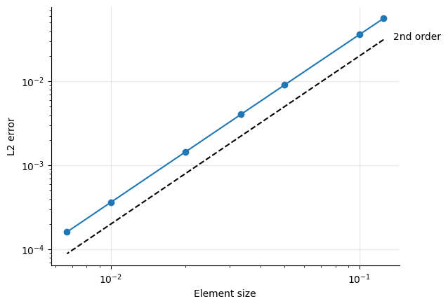
It is also possible to compute how the numerical error decreases as we increase the number of cells. By iteratively refining the mesh, we find that the error exhibits a second order convergence rate. This is expected for this particular problem as first order finite elements are used.
import matplotlib.pyplot as plt

errors = []
ns = [8, 10, 20, 30, 50, 100, 150]

for n in ns:
    nx = ny = n
    fenics_mesh = dolfinx.mesh.create_unit_square(MPI.COMM_WORLD, nx, ny)

    new_model = F.HeatTransferProblem()
    new_model.mesh = F.Mesh(fenics_mesh)

    new_model.subdomains = my_model.subdomains
    new_model.sources = my_model.sources
    new_model.boundary_conditions = my_model.boundary_conditions
    new_model.settings = my_model.settings

    new_model.initialise()
    new_model.run()

    computed_solution = new_model.u
    errors.append(error_L2(computed_solution, exact_solution(np)))

h = 1 / np.array(ns)

plt.loglog(h, errors, marker="o")
plt.xlabel("Element size")
plt.ylabel("L2 error")

plt.loglog(h, 2 * h**2, linestyle="--", color="black")
plt.annotate(
    "2nd order", (h[0], 2 * h[0] ** 2), textcoords="offset points", xytext=(10, 0)
)

plt.grid(alpha=0.3)
plt.gca().spines[["right", "top"]].set_visible(False)
plt.show()