Diffusion through a semi-infinite slab

🏷 Tags: 1D MES transient

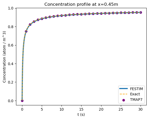
This verification case from TMAP7’s V&V report [3] consists of a semi-infinite slab with no traps under a constant concentration \(C_0\) boundary condition on the left.

FESTIM Code

import festim as F

from dolfinx.geometry import bb_tree, compute_colliding_cells, compute_collisions_points


class PointValue(F.VolumeQuantity):
    def __init__(self, field, volume, x0, filename=None):
        super().__init__(field, volume, filename)
        self.x0 = x0

    def compute(self):
        u = self.field.solution
        mesh = u.function_space.mesh
        tree = bb_tree(mesh, mesh.geometry.dim)
        cell_candidates = compute_collisions_points(tree, self.x0)
        cell = compute_colliding_cells(mesh, cell_candidates, self.x0).array
        assert len(cell) > 0
        first_cell = cell[0]

        self.value = self.field.solution.eval(self.x0, first_cell)
        self.data.append(self.value)

/home/docs/checkouts/readthedocs.org/user_builds/festim-vv-report/conda/festim-2/lib/python3.11/site-packages/festim/coupled_heat_hydrogen_problem.py:1: TqdmExperimentalWarning: Using `tqdm.autonotebook.tqdm` in notebook mode. Use `tqdm.tqdm` instead to force console mode (e.g. in jupyter console)
  import tqdm.autonotebook

Show code cell content

Hide code cell content

import festim as F
import numpy as np
from scipy.special import erf
from matplotlib import pyplot as plt

C_0 = 1  # atom m^-3
D = 1  # m^2 s^-1
exact_solution = lambda x, t: C_0 * (1 - erf(x / np.sqrt(4 * D * t)))

model = F.HydrogenTransportProblem()

### Mesh Settings ###
vertices = np.concatenate(
    [
        np.linspace(0, 1, 100),
        np.linspace(1, 20, 200),
        np.linspace(20, 200, 200),
    ]
)

model.mesh = F.Mesh1D(vertices)

material = F.Material(D_0=D, E_D=0)

left_surface = F.SurfaceSubdomain1D(id=1, x=0)
volume = F.VolumeSubdomain1D(id=2, borders=[0, 200], material=material)
model.subdomains = [left_surface, volume]

H = F.Species("H")
model.species = [H]


model.boundary_conditions = [
    F.FixedConcentrationBC(subdomain=left_surface, value=C_0, species=H)
]


model.temperature = 500.0  # ignored in this problem

model.settings = F.Settings(atol=1e-10, rtol=1e-10, final_time=30)

model.settings.stepsize = F.Stepsize(
    initial_value=0.005,
    growth_factor=1.1,
    cutback_factor=0.9,
    target_nb_iterations=4,
    milestones=[model.settings.final_time],
)


test_point_x = 0.45
point_value = PointValue(model.species[0], volume=volume, x0=np.array([test_point_x, 0, 0]))

model.exports = [point_value]

model.initialise()
model.run()

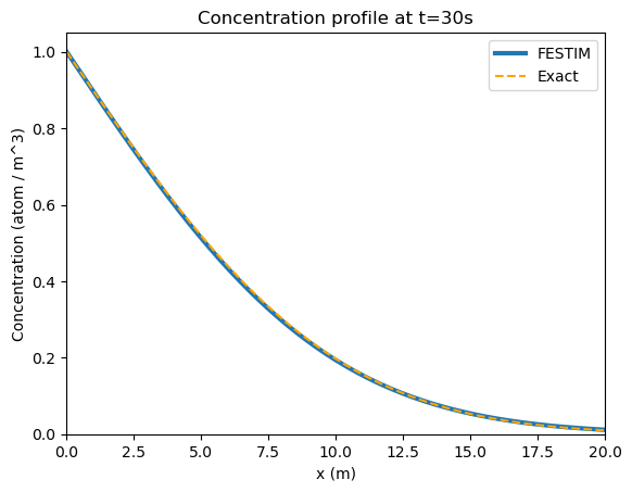
Comparison with exact solution

The exact solution is given by

\[ c(x, t) = c_0 \left( 1 - \mathrm{erf}\left( \frac{x}{2\sqrt{Dt}} \right) \right) \]

Show code cell source

Hide code cell source

# plotting computed data
computed_solution = H.solution.x.array[:]
computed_x = model.mesh.mesh.geometry.x[:, 0]
plt.plot(computed_x, computed_solution, label="FESTIM", linewidth=3)

# plotting exact solution
exact_y = exact_solution(np.array(computed_x), model.settings.final_time)
plt.plot(computed_x, exact_y, label="Exact", color="orange", linestyle="--")

plt.title(f"Concentration profile at t={model.settings.final_time}s")
plt.ylabel("Concentration (atom / m^3)")
plt.xlabel("x (m)")
plt.ylim(bottom=0)

plt.xlim(0, 20)  # since it's semi infinite, zoom in

plt.legend()
plt.show()

Show code cell source

Hide code cell source

# plotting computed data
computed_solution = point_value.data
t = point_value.t
plt.plot(t, computed_solution, label="FESTIM", linewidth=3)

# plotting exact solution
exact_y = exact_solution(test_point_x, np.array(t))

plt.plot(t, exact_y, label="Exact", color="orange", linestyle="--")

# plotting TMAP data
tmap_data = np.genfromtxt("./tmap_point_data.txt", delimiter=" ", names=True)
tmap_t = tmap_data["t"]
tmap_solution = tmap_data["tmap"]
plt.scatter(tmap_t, tmap_solution, label="TMAP7", color="purple")

plt.title(f"Concentration profile at x={test_point_x}m")
plt.ylabel("Concentration (atom / m^3)")
plt.xlabel("t (s)")

plt.legend()
plt.show()