Diffusion multi-material

🏷 Tags: 2D MMS Multi-material steady state

The first MMS problem has two materials (denoted, respectively, by left and right). In material left, the solubility is \(K_{S,\mathrm{left}} = 3\) and the diffusivity is \(D_\mathrm{left} = 2\). In material right, the solubility is \(K_{S,\mathrm{right}} = 6\) and the diffusivity is \(D_\mathrm{right} = 5\). Two exact solutions for mobile concentration of hydrogen are manufactured for both subdomains:

(16)\[\begin{align} c_\mathrm{left,exact} &= 1 + \sin{\left(\pi \left(2 x + 0.5\right) \right)} + \cos{\left(2 \pi y \right)} \\ c_\mathrm{right,exact} &= \dfrac{K_{S,\mathrm{right}}}{K_{S,\mathrm{left}}} \ c_\mathrm{left,exact} \end{align}\]

Note

The manufactured solutions were chosen so that the particle flux \(J = -D \nabla c_\mathrm{m} \cdot \textbf{n}\) is continuous across the materials interface.

MMS sources are derived in each material:

(17)\[\begin{align} S_\mathrm{left} &= 8 \pi^{2} \left(\cos{\left(2 \pi x \right)} + \cos{\left(2 \pi y \right)}\right) \\ S_\mathrm{right} &= 40 \pi^{2} \left(\cos{\left(2 \pi x \right)} + \cos{\left(2 \pi y \right)}\right) \end{align}\]

These exact solutions can then determine the MMS fluxes and boundary conditions.

FESTIM code

Show code cell source

Hide code cell source

import festim as F
import numpy as np
import dolfinx
import ufl
from mpi4py import MPI

# Create and mark the mesh
nx = ny = 10
fenics_mesh = dolfinx.mesh.create_unit_square(MPI.COMM_WORLD, nx, ny)


class LeftSurface(F.SurfaceSubdomain):
    def locate_boundary_facet_indices(self, mesh):
        return dolfinx.mesh.locate_entities_boundary(
            mesh, mesh.topology.dim - 1, lambda x: np.isclose(x[0], 0.0)
        )


class RightSurface(F.SurfaceSubdomain):
    def locate_boundary_facet_indices(self, mesh):
        return dolfinx.mesh.locate_entities_boundary(
            mesh, mesh.topology.dim - 1, lambda x: np.isclose(x[0], 1.0)
        )


class TopRightSurface(F.SurfaceSubdomain):
    def locate_boundary_facet_indices(self, mesh):
        return dolfinx.mesh.locate_entities_boundary(
            mesh, mesh.topology.dim - 1, lambda x: np.isclose(x[1], 1.0) & (x[0] > 0.5)
        )


class TopLeftSurface(F.SurfaceSubdomain):
    def locate_boundary_facet_indices(self, mesh):
        return dolfinx.mesh.locate_entities_boundary(
            mesh, mesh.topology.dim - 1, lambda x: np.isclose(x[1], 1.0) & (x[0] < 0.5)
        )


class BottomRightSurface(F.SurfaceSubdomain):
    def locate_boundary_facet_indices(self, mesh):
        return dolfinx.mesh.locate_entities_boundary(
            mesh, mesh.topology.dim - 1, lambda x: np.isclose(x[1], 0.0) & (x[0] > 0.5)
        )


class BottomLeftSurface(F.SurfaceSubdomain):
    def locate_boundary_facet_indices(self, mesh):
        return dolfinx.mesh.locate_entities_boundary(
            mesh, mesh.topology.dim - 1, lambda x: np.isclose(x[1], 0.0) & (x[0] < 0.5)
        )


class LeftSubdomain(F.VolumeSubdomain):
    def locate_subdomain_entities(self, mesh):
        return dolfinx.mesh.locate_entities(
            mesh, mesh.topology.dim, lambda x: x[0] < 0.5 + 1e-10
        )


class RightSubdomain(F.VolumeSubdomain):
    def locate_subdomain_entities(self, mesh):
        return dolfinx.mesh.locate_entities(
            mesh, mesh.topology.dim, lambda x: x[0] >= 0.5 - 1e-10
        )


left_surface = LeftSurface(id=1)
right_surface = RightSurface(id=2)
top_left_surface = TopLeftSurface(id=3)
bottom_left_surface = BottomLeftSurface(id=4)
top_right_surface = TopRightSurface(id=5)
bottom_right_surface = BottomRightSurface(id=6)


# Create the FESTIM model
my_model = F.HydrogenTransportProblemDiscontinuous()

my_model.mesh = F.Mesh(fenics_mesh)

D_left, D_right = 2, 5  # diffusion coeffs
S_left = 3
S_right = 6

mat_left = F.Material(D_0=D_left, E_D=0, K_S_0=S_left, E_K_S=0)
mat_right = F.Material(D_0=D_right, E_D=0, K_S_0=S_right, E_K_S=0)
left_volume = LeftSubdomain(id=1, material=mat_left)
right_volume = RightSubdomain(id=2, material=mat_right)

my_model.subdomains = [
    left_volume,
    right_volume,
    left_surface,
    right_surface,
    top_left_surface,
    bottom_left_surface,
    top_right_surface,
    bottom_right_surface,
]

my_model.surface_to_volume = {
    left_surface: left_volume,
    right_surface: right_volume,
    top_left_surface: left_volume,
    bottom_left_surface: left_volume,
    top_right_surface: right_volume,
    bottom_right_surface: right_volume,
}

my_model.interfaces = [F.Interface(id=7, subdomains=[left_volume, right_volume])]

H = F.Species("H", subdomains=my_model.volume_subdomains)
my_model.species = [H]


def exact_solution_left(mod):
    return lambda x: (
        1 + mod.sin(2 * mod.pi * (x[0] + 0.25)) + mod.cos(2 * mod.pi * x[1])
    )


def exact_solution_right(mod):
    return lambda x: S_right / S_left * exact_solution_left(mod)(x)


exact_solution_left_ufl = exact_solution_left(ufl)
exact_solution_right_ufl = exact_solution_right(ufl)


# source terms
f_left = lambda x: -ufl.div(D_left * ufl.grad(exact_solution_left_ufl(x)))
f_right = lambda x: -ufl.div(D_right * ufl.grad(exact_solution_right_ufl(x)))


my_model.sources = [
    F.ParticleSource(f_left, volume=left_volume, species=H),
    F.ParticleSource(f_right, volume=right_volume, species=H),
]

# boundary conditions
my_model.boundary_conditions = [
    F.FixedConcentrationBC(subdomain=surface, value=exact_solution_left_ufl, species=H)
    for surface in [left_surface, top_left_surface, bottom_left_surface]
] + [
    F.FixedConcentrationBC(subdomain=surface, value=exact_solution_right_ufl, species=H)
    for surface in [right_surface, top_right_surface, bottom_right_surface]
]


my_model.temperature = 500.0

my_model.settings = F.Settings(atol=1e-10, rtol=1e-10, transient=False)

my_model.initialise()
my_model.run()

Show code cell output

Hide code cell output

/home/docs/checkouts/readthedocs.org/user_builds/festim-vv-report/conda/festim-2/lib/python3.11/site-packages/festim/coupled_heat_hydrogen_problem.py:1: TqdmExperimentalWarning: Using `tqdm.autonotebook.tqdm` in notebook mode. Use `tqdm.tqdm` instead to force console mode (e.g. in jupyter console)
  import tqdm.autonotebook

Comparison with exact solution

The concentration fields can be visualised using pyvista.

import pyvista
from dolfinx.plot import vtk_mesh

pyvista.start_xvfb()
pyvista.set_jupyter_backend("html")


def get_ugrid(computed_solution: dolfinx.fem.Function, label):
    u_topology, u_cell_types, u_geometry = vtk_mesh(computed_solution.function_space)
    u_grid = pyvista.UnstructuredGrid(u_topology, u_cell_types, u_geometry)
    u_grid.point_data[label] = computed_solution.x.array.real
    u_grid.set_active_scalars(label)
    return u_grid


u_plotter = pyvista.Plotter(shape=(1, 2))
u_grid_left = get_ugrid(H.subdomain_to_post_processing_solution[left_volume], "c")
u_grid_right = get_ugrid(H.subdomain_to_post_processing_solution[right_volume], "c")

u_plotter.subplot(0, 0)
u_plotter.add_mesh(u_grid_left, show_edges=True)
u_plotter.add_mesh(u_grid_right, show_edges=True)
u_plotter.view_xy()

u_plotter.subplot(0, 1)
exact_left = dolfinx.fem.Function(
    H.subdomain_to_post_processing_solution[left_volume].function_space
)
exact_left.interpolate(exact_solution_left(np))
exact_right = dolfinx.fem.Function(
    H.subdomain_to_post_processing_solution[right_volume].function_space
)
exact_right.interpolate(exact_solution_right(np))
u_grid_exact_left = get_ugrid(exact_left, "c_exact")
u_grid_exact_right = get_ugrid(exact_right, "c_exact")


u_plotter.add_mesh(u_grid_exact_left, show_edges=False)
u_plotter.add_mesh(u_grid_exact_right, show_edges=False)
u_plotter.view_xy()

if not pyvista.OFF_SCREEN:
    u_plotter.show()
else:
    figure = u_plotter.screenshot("discontinuity_concentration.png")

/home/docs/checkouts/readthedocs.org/user_builds/festim-vv-report/conda/festim-2/lib/python3.11/site-packages/pyvista/plotting/utilities/xvfb.py:48: PyVistaDeprecationWarning: This function is deprecated and will be removed in future version of PyVista. Use vtk-osmesa instead.
  warnings.warn(

Computing errors

First, we compute the \(L^2\)-norm of the error, defined by \(E=\sqrt{\int_\Omega (c-c_\mathrm{exact})^2\mathrm{d} x}\). Secondly, we compute the maximum error at any degree of freedom.

Show code cell source

Hide code cell source

def error_L2(u_computed, u_exact, degree_raise=3):
    # Create higher order function space
    degree = u_computed.function_space.ufl_element().degree
    family = u_computed.function_space.ufl_element().family_name
    mesh = u_computed.function_space.mesh
    W = dolfinx.fem.functionspace(mesh, (family, degree + degree_raise))

    # Interpolate exact solution, special handling if exact solution
    # is a ufl expression or a python lambda function
    u_ex_W = dolfinx.fem.Function(W)
    if isinstance(u_exact, ufl.core.expr.Expr):
        u_expr = dolfinx.fem.Expression(u_exact, W.element.interpolation_points)
        u_ex_W.interpolate(u_expr)
    else:
        u_ex_W.interpolate(u_exact)

    # Integrate the error
    error = dolfinx.fem.form(
        ufl.inner(u_computed - u_ex_W, u_computed - u_ex_W) * ufl.dx
    )
    error_local = dolfinx.fem.assemble_scalar(error)
    error_global = mesh.comm.allreduce(error_local, op=MPI.SUM)
    return np.sqrt(error_global)

computed_left = H.subdomain_to_post_processing_solution[left_volume]
computed_right = H.subdomain_to_post_processing_solution[right_volume]

E_l2_left = error_L2(computed_left, exact_solution_left(np))
E_max_left = np.max(np.abs(exact_left.x.array - computed_left.x.array))
E_l2_right = error_L2(computed_right, exact_solution_right(np))
E_max_right = np.max(np.abs(exact_right.x.array - computed_right.x.array))

print("Left volume:")
print(f"L2 error: {E_l2_left:.2e}")
print(f"Max error: {E_max_left:.2e}")

print("\nRight volume:")
print(f"L2 error: {E_l2_right:.2e}")
print(f"Max error: {E_max_right:.2e}")

Left volume:
L2 error: 2.78e-02
Max error: 5.63e-02

Right volume:
L2 error: 5.26e-02
Max error: 7.25e-02

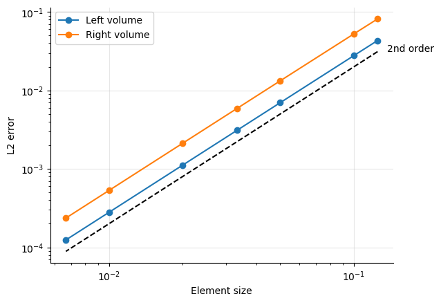
Compute convergence rates

It is also possible to compute how the numerical error decreases as we increase the number of cells. By iteratively refining the mesh, we find that the error exhibits a second order convergence rate. This is expected for this particular problem as first order finite elements are used.

import matplotlib.pyplot as plt

errors_left, errors_right = [], []
ns = [8, 10, 20, 30, 50, 100, 150]

for n in ns:
    nx = ny = n
    fenics_mesh = dolfinx.mesh.create_unit_square(MPI.COMM_WORLD, nx, ny)

    new_model = F.HydrogenTransportProblemDiscontinuous()
    new_model.mesh = F.Mesh(fenics_mesh)

    new_model.species = my_model.species
    new_model.subdomains = my_model.subdomains
    new_model.surface_to_volume = my_model.surface_to_volume
    new_model.interfaces = my_model.interfaces
    new_model.sources = my_model.sources
    new_model.boundary_conditions = my_model.boundary_conditions
    new_model.temperature = my_model.temperature
    new_model.settings = my_model.settings


    new_model.initialise()
    new_model.run()

    computed_solution_left = H.subdomain_to_post_processing_solution[left_volume]
    computed_solution_right = H.subdomain_to_post_processing_solution[right_volume]
    errors_left.append(error_L2(computed_solution_left, exact_solution_left(np)))
    errors_right.append(error_L2(computed_solution_right, exact_solution_right(np)))

h = 1 / np.array(ns)

plt.loglog(h, errors_left, marker="o", label="Left volume")
plt.loglog(h, errors_right, marker="o", label="Right volume")
plt.xlabel("Element size")
plt.ylabel("L2 error")

plt.loglog(h, 2 * h**2, linestyle="--", color="black")
plt.annotate(
    "2nd order", (h[0], 2 * h[0] ** 2), textcoords="offset points", xytext=(10, 0)
)

plt.grid(alpha=0.3)
plt.gca().spines[["right", "top"]].set_visible(False)
plt.legend()
plt.show()