Diffusion with Composite Material Layers

🏷 Tags: 1D MES transient

This verification case is Val-1e of TMAP7’s V&V report [3]. It consists of a composite one-dimensional domain with two materials (PyC and SiC) without traps and the fixed concentration on the left boundary. The concentration at the opposite side is equal to zero.

The problem can be analytically solved. The steady state solution for the PyC is given in [3] as:

\[ C = C_0 \left[1 + \frac{x}{l} \left(\frac{a D_{PyC}}{a D_{PyC} + l D_{SiC}} - 1 \right) \right] \]

while the concentration profile for the SiC layer is given as:

\[ C = C_0 \left(\frac{a+l-x}{l} \right) \left(\frac{a D_{PyC}}{a D_{PyC} + l D_{SiC}} \right) \]

where

\(x\) is the distance from free surface of PyC

\(a\) is the thickness of the PyC layer (\(33 \ \mathrm{\mu m}\))

\(l\) is the thickness of the SiC layer (\(66 \ \mathrm{\mu m}\))

\(C_0\) is the concentration at the PyC free surface (\(3.0537 \times 10^{25} \mathrm{m}^{-3}\))

\(D_{PyC}\) is the diffusivity in PyC (\(1.274 \times 10^{-7}~\mathrm{m}^{2}\mathrm{s}^{-1}\))

\(D_{SiC}\) is the diffusivity in SiC (\(2.622 \times 10^{-11}~\mathrm{m}^{2}\mathrm{s}^{-1}\))

The analytical transient solution from Table 3, row 1 in [10] for the concentration in the PyC and SiC side of the composite slab is given as:

\[ C = C_0 \left\{ \frac{(a-x) D_{SiC} + l D_{PyC}}{l D_{PyC} + a D_{SiC}} + 2 \sum_{n=1}^{\infty} B_n \sin\left(\lambda_n \frac{x}{a}\right) \exp\left(-D_{PyC} \frac{\lambda^2_n}{a^2} t \right) \right\} \]

and

\[ C = C_0 \left\{ \frac{(l+a-x) D_{PyC}}{l D_{PyC} + a D_{SiC}} + 2 \sum_{n=1}^{\infty} B_n \frac{\sin(\lambda_n)}{\sin(k \lambda_n l/a)} \sin\left(k \lambda_n \frac{l+a-x}{a}\right) \exp\left(-D_{PyC} \frac{\lambda^2_n}{a^2} t \right) \right\} \]

where

\[ k = \sqrt{\frac{D_{PyC}}{D_{SiC}}}, \]

\[ B_n = \frac{D_{PyC} l \sin^2(k \lambda_n l/a) (\cos(\lambda_n) - 1) + D_{SiC} \sin(k \lambda_n l/a) (k l \sin(\lambda_n) \cos(k \lambda_n l/a) - a \sin(k \lambda_n l/a))}{ \lambda_n (a D_{SiC} + l D_{PyC}) (\sin^2(k \lambda_n l/a) + (l/a) \sin^2(\lambda_n))}, \]

and \(\lambda_n\) are the roots of

\[ \frac{\sin(\lambda_n) \cos(k \lambda_n l/a)}{k} + \cos(\lambda_n) \sin(k \lambda_n l/a) = 0. \]

Note

In TMAP8 V&V there is a note stating that the expressions of the analytical solution for the transient case in TMAP4 and TMAP7 V&V books are inconsistent with the results, which suggest typographical errors. Therefore, we used the expression provided in TMAP8 V&V and taken from [10].

FESTIM Code

import festim as F
import numpy as np

from dolfinx.geometry import bb_tree, compute_colliding_cells, compute_collisions_points


class PointValue(F.VolumeQuantity):
    def __init__(self, field, volume, x0, filename=None):
        super().__init__(field, volume, filename)
        self.x0 = x0

    def compute(self):
        u = self.field.solution
        mesh = u.function_space.mesh
        tree = bb_tree(mesh, mesh.geometry.dim)
        cell_candidates = compute_collisions_points(tree, self.x0)
        cell = compute_colliding_cells(mesh, cell_candidates, self.x0).array
        assert len(cell) > 0
        first_cell = cell[0]

        self.value = self.field.solution.eval(self.x0, first_cell)
        self.data.append(self.value)


# Define input parameters
a = 33e-6
l = 66e-6
D0_PyC = 1.274e-7
D0_SiC = 2.622e-11
T = 1.0e3
c_left = 3.0537e25

# Create the FESTIM model
model = F.HydrogenTransportProblem()

vertices = np.concatenate(
    [
        np.linspace(0, a, num=500),
        np.linspace(a, a + l, num=500),
    ]
)

model.mesh = F.Mesh1D(vertices)

material_PyC = F.Material(D_0=D0_PyC, E_D=0)
material_SiC = F.Material(D_0=D0_SiC, E_D=0)

left_volume = F.VolumeSubdomain1D(id=1, borders=[0, a], material=material_PyC)
right_volume = F.VolumeSubdomain1D(id=2, borders=[a, a + l], material=material_SiC)
left_surface = F.SurfaceSubdomain1D(id=3, x=0)
right_surface = F.SurfaceSubdomain1D(id=4, x=a + l)

model.subdomains = [left_volume, right_volume, left_surface, right_surface]

H = F.Species("H")
model.species = [H]

model.temperature = T

model.boundary_conditions = [
    F.FixedConcentrationBC(subdomain=left_surface, value=c_left, species=H),
    F.FixedConcentrationBC(subdomain=right_surface, value=0, species=H),
]

model.settings = F.Settings(atol=1e10, rtol=1e-10, max_iterations=30, final_time=100)
model.settings.stepsize = F.Stepsize(
    initial_value=1e-4,
    growth_factor=1.1,
    cutback_factor=0.9,
    target_nb_iterations=10,
    max_stepsize=1,
)

x1 = 32e-6
x2 = 48.75e-6

point_value1 = PointValue(model.species[0], volume=left_volume, x0=np.array([x1, 0, 0]))
point_value2 = PointValue(
    model.species[0], volume=right_volume, x0=np.array([x2, 0, 0])
)

model.exports = [point_value1, point_value2]

model.initialise()
model.run()

/home/docs/checkouts/readthedocs.org/user_builds/festim-vv-report/conda/festim-2/lib/python3.11/site-packages/festim/coupled_heat_hydrogen_problem.py:1: TqdmExperimentalWarning: Using `tqdm.autonotebook.tqdm` in notebook mode. Use `tqdm.tqdm` instead to force console mode (e.g. in jupyter console)
  import tqdm.autonotebook

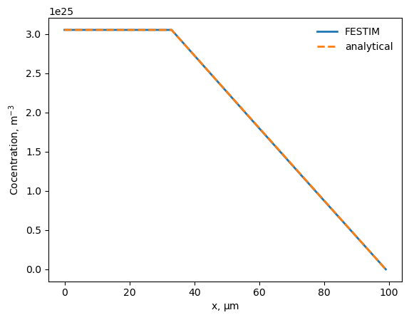
Comparison with exact solution

Show code cell source

Hide code cell source

def analytical_expression_steadystate(x_mesh, a, l, D0_PyC, D0_SiC):
    """
    Analytical expression for the steady state hydrogen depth distribution

    Args:
        x_mesh (ndarray): array of mesh coordinates in meters
        a (float): length of the PyC layer (m)
        l (float): length of the SiC layer (m)
        D0_PyC (float): H diffusivity in PyC (m^2 s^-1)
        D0_SiC (float): H diffusivity in SiC (m^2 s^-1)

    Returns:
        np.array: array of concentration values
    """

    c_exact = np.zeros_like(x_mesh)
    for i, x in enumerate(x_mesh):
        if x <= a:
            c_exact[i] = c_left * (
                1 + x / l * (a * D0_PyC / (a * D0_PyC + l * D0_SiC) - 1)
            )
        else:
            c_exact[i] = (
                c_left * (a + l - x) / (l) * a * D0_PyC / (a * D0_PyC + l * D0_SiC)
            )

    return c_exact


def RMSPE(x_FESTIM, x_analytical):
    error = (
        np.sqrt(np.mean((x_FESTIM - x_analytical) ** 2)) * 100 / np.mean(x_analytical)
    )
    return error

import matplotlib.pyplot as plt

computed_solution = H.solution.x.array[:]
computed_x = model.mesh.mesh.geometry.x[:, 0]
analytical_solution = analytical_expression_steadystate(
    computed_x, a, l, D0_PyC, D0_SiC
)

error = RMSPE(computed_solution, analytical_solution)
print(f"RMSPE={error:.2f}%")

plt.plot(computed_x * 1e6, computed_solution, label="FESTIM", linewidth=2)
plt.plot(
    computed_x * 1e6, analytical_solution, label="analytical", linewidth=2, ls="dashed"
)


plt.ylabel(r"Cocentration, m$^{-3}$")
plt.xlabel(r"x, $\mathrm{\mu}$m")
plt.legend(frameon=False)
plt.show()

RMSPE=0.12%

Show code cell source

Hide code cell source

def get_lambdas_analytical(k, l, a):
    # Calculate lambda values for analytical solution
    # The function was taken from TMAP8 V&V https://github.com/idaholab/TMAP8/blob/de10192998e63dfedfdd260e86a1d7726f765303/test/tests/ver-1e/comparison_ver-1e.py#L13-L20
    lambda_range = np.arange(1e-12, 1e2, 1e-5)
    f = 1 / k * np.sin(lambda_range) * np.cos(lambda_range * l / a * k)
    g = np.cos(lambda_range) * np.sin(lambda_range * l / a * k)
    idx = np.where(np.diff(np.sign(f + g)))
    lambdas = lambda_range[idx][::1]
    return lambdas


def analytical_expression_temporal(t, x, a, l, D0_PyC, D0_SiC):
    """Analytical expression for the temporal dependency of the hydrogen concentration at a given point

    Args:
        t (ndarray): array of times
        x (float): mesh coordinate (m)
        a (float): length of the PyC layer (m)
        l (float): length of the SiC layer (m)
        D0_PyC (float): H diffusivity in PyC (m^2 s^-1)
        D0_SiC (float): H diffusivity in SiC (m^2 s^-1)

    Returns:
        np.array: array of concentration values
    """

    k = np.sqrt(D0_PyC / D0_SiC)
    f = l / a

    roots = get_lambdas_analytical(k, l, a)
    roots = roots[:, np.newaxis]

    sinus1 = np.sin(k * roots * f)
    cosinus1 = np.cos(k * roots * f)
    Bn = (
        D0_PyC * l * sinus1**2 * (np.cos(roots) - 1)
        + D0_SiC * sinus1 * (k * l * np.sin(roots) * cosinus1 - a * sinus1)
    ) / (roots * (a * D0_SiC + l * D0_PyC) * (sinus1**2 + f * np.sin(roots) ** 2))

    sum = 0
    if x <= a:
        sum = Bn * np.sin(roots * x / a) * np.exp(-D0_PyC * (roots / a) ** 2 * t)
        sum = np.sum(sum, axis=0)
        c_exact = c_left * (
            ((a - x) * D0_SiC + l * D0_PyC) / (l * D0_PyC + a * D0_SiC) + 2 * sum
        )
    else:
        sum = (
            Bn
            * np.sin(roots)
            / sinus1
            * np.sin(k * roots * (a + l - x) / a)
            * np.exp(-D0_PyC * (roots / a) ** 2 * t)
        )
        sum = np.sum(sum, axis=0)
        c_exact = c_left * (D0_PyC * (a + l - x) / (l * D0_PyC + a * D0_SiC) + 2 * sum)

    return c_exact

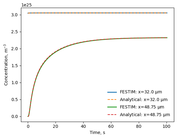
for x, festim_data in zip([x1, x2], [point_value1, point_value2]):
    t = np.array(festim_data.t)
    indx = np.where(t >= 0.1)[0]
    t = t[indx]
    festim_solution = np.array(festim_data.data)[indx].flatten()

    analytical_solution = analytical_expression_temporal(t, x, a, l, D0_PyC, D0_SiC)

    error = RMSPE(festim_solution, analytical_solution)
    print(f"RMSPE at x={x} m is {error:.2f}%")

    plt.plot(
        t, festim_solution, label=f"FESTIM: x={x*1e6}" + r" $\mathrm{\mu m}$", lw=2
    )
    plt.plot(
        t,
        analytical_solution,
        ls="dashed",
        label=f"Analytical: x={x*1e6}" + r" $\mathrm{\mu m}$",
    )

plt.ylabel(r"Concentration, m$^{-3}$")
plt.xlabel("Time, s")
plt.legend(frameon=False)
plt.show()

RMSPE at x=3.2e-05 m is 0.04%

RMSPE at x=4.875e-05 m is 0.54%