Radioactive decay 1D#
This example is a radioactive decay problem on simple unit interval with a uniform mobile concentration and no boundary condition.
In this problem, for simplicity, we don’t set any traps and we model an isolated domain (no flux boundary conditions) to mimick a simple 0D case. Diffusion can therefore be neglected and the problem is:
The exact solution for mobile concentration is:
Here, \(c_0\) is the initial concentration and \(\lambda\) is the decay constant (in \(s^{-1}\)). We can then run a FESTIM model with these conditions and compare the numerical solution with \(c_\mathrm{exact}\).
We can then run a FESTIM model with these conditions and compare the numerical solution with \(c_\mathrm{exact}\).
FESTIM Code#
import festim as F
import numpy as np
import matplotlib.pyplot as plt
initial_concentration = 3.0
def run_model(half_life):
my_model = F.HydrogenTransportProblem()
my_model.mesh = F.Mesh1D(np.linspace(0, 1, 1001))
my_mat = F.Material(D_0=1, E_D=0)
volume = F.VolumeSubdomain1D(id=1, borders=[0, 1], material=my_mat)
left_boundary = F.SurfaceSubdomain1D(id=1, x=0)
right_boundary = F.SurfaceSubdomain1D(id=2, x=1)
my_model.subdomains = [volume, left_boundary, right_boundary]
H = F.Species("H")
my_model.species = [H]
decay_constant = np.log(2) / half_life
decay_reaction = F.Reaction(reactant=H, k_0=decay_constant, E_k=0, volume=volume)
my_model.reactions = [decay_reaction]
my_model.temperature = 300 # ignored in this problem
average_volume = F.AverageVolume(field=H, volume=volume)
my_model.exports = [average_volume]
my_model.initial_conditions = [F.InitialConcentration(value=initial_concentration, species=H, volume=volume)]
my_model.settings = F.Settings(
atol=1e-10, rtol=1e-10, final_time=5 * half_life, transient=True
)
my_model.settings.stepsize = F.Stepsize(
initial_value=0.05,
growth_factor=1.01,
cutback_factor=0.99,
target_nb_iterations=4,
)
my_model.initialise()
my_model.run()
time = average_volume.t
concentration = average_volume.data
return time, concentration
tests = []
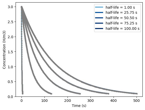
for half_life in np.linspace(1, 100, 5):
tests.append((*run_model(half_life), half_life))
/home/docs/checkouts/readthedocs.org/user_builds/festim-vv-report/conda/festim-2/lib/python3.11/site-packages/festim/coupled_heat_hydrogen_problem.py:1: TqdmExperimentalWarning: Using `tqdm.autonotebook.tqdm` in notebook mode. Use `tqdm.tqdm` instead to force console mode (e.g. in jupyter console)
  import tqdm.autonotebook
Comparison with exact solution#
The evolution of the hydrogen concentration is computed with FESTIM and compared with the exact solution (shown in dashed lines).