Diffusion multi-material

Diffusion multi-material#

🏷 Tags: 2D MMS Multi-material steady state

The first MMS problem has two materials (denoted, respectively, by left and right). In material left, the solubility is \(K_{S,\mathrm{left}} = 3\) and the diffusivity is \(D_\mathrm{left} = 2\). In material right, the solubility is \(K_{S,\mathrm{right}} = 6\) and the diffusivity is \(D_\mathrm{right} = 5\). Two exact solutions for mobile concentration of hydrogen are manufactured for both subdomains:

(16)#\[\begin{align} c_\mathrm{left,exact} &= 1 + \sin{\left(\pi \left(2 x + 0.5\right) \right)} + \cos{\left(2 \pi y \right)} \\ c_\mathrm{right,exact} &= \dfrac{K_{S,\mathrm{right}}}{K_{S,\mathrm{left}}} \ c_\mathrm{left,exact} \end{align}\]

MMS sources are derived in each material:

(17)#\[\begin{align} S_\mathrm{left} &= 8 \pi^{2} \left(\cos{\left(2 \pi x \right)} + \cos{\left(2 \pi y \right)}\right) \\ S_\mathrm{right} &= 40 \pi^{2} \left(\cos{\left(2 \pi x \right)} + \cos{\left(2 \pi y \right)}\right) \end{align}\]

These exact solutions can then determine the MMS fluxes and boundary conditions.

FESTIM code#

Show code cell source Hide code cell source

import festim as F
import sympy as sp
import fenics as f
import matplotlib as mpl
import matplotlib.pyplot as plt
import numpy as np

# Create and mark the mesh

fenics_mesh = f.UnitSquareMesh(100, 100)

left_surface = f.CompiledSubDomain("near(x[0], 0.0)")
right_surface = f.CompiledSubDomain("near(x[0], 1.0)")
top_right_surface = f.CompiledSubDomain("near(x[1], 1.0) && x[0] > 0.5")
top_left_surface = f.CompiledSubDomain("near(x[1], 1.0) && x[0] < 0.5")
bottom_right_surface = f.CompiledSubDomain("near(x[1], 0.0) && x[0] > 0.5")
bottom_left_surface = f.CompiledSubDomain("near(x[1], 0.0) && x[0] < 0.5")


class LeftSubdomain(f.SubDomain):
    def inside(self, x, on_boundary):
        return f.between(x[0], (0.0, 0.5))


class RightSubdomain(f.SubDomain):
    def inside(self, x, on_boundary):
        return f.between(x[0], (0.5, 1.0))


volume_markers = f.MeshFunction("size_t", fenics_mesh, fenics_mesh.topology().dim())
volume_markers.set_all(0)
left_volume = LeftSubdomain()
right_volume = RightSubdomain()

left_volume.mark(volume_markers, 1)
right_volume.mark(volume_markers, 2)

surface_markers = f.MeshFunction(
    "size_t", fenics_mesh, fenics_mesh.topology().dim() - 1
)
surface_markers.set_all(0)
left_surface.mark(surface_markers, 1)
top_left_surface.mark(surface_markers, 2)
top_right_surface.mark(surface_markers, 3)
right_surface.mark(surface_markers, 4)
bottom_right_surface.mark(surface_markers, 5)
bottom_left_surface.mark(surface_markers, 6)

# Create the FESTIM model
my_model = F.Simulation()

my_model.mesh = F.Mesh(
    fenics_mesh, volume_markers=volume_markers, surface_markers=surface_markers
)

# Variational formulation
x = F.x
y = F.y

S_left = 3
S_right = 6

exact_solution_left = (
    1 + sp.sin(2 * sp.pi * (x + 0.25)) + sp.cos(2 * sp.pi * y)
)  # exact solution
exact_solution_right = S_right / S_left * exact_solution_left

D_left, D_right = 2, 5  # diffusion coeffs


def grad(u):
    """Computes the gradient of a function u.

    Args:
        u (sympy.Expr): a sympy function

    Returns:
        sympy.Matrix: the gradient of u
    """
    return sp.Matrix([sp.diff(u, x), sp.diff(u, y)])


def div(u):
    """Computes the divergence of a vector field u.

    Args:
        u (sympy.Matrix): a sympy vector field

    Returns:
        sympy.Expr: the divergence of u
    """
    return sp.diff(u[0], x) + sp.diff(u[1], y)


# source term left
f_left = -div(D_left * grad(exact_solution_left))
f_right = -div(D_right * grad(exact_solution_right))


print(
    f"Source term left: {sp.latex(f_left.simplify().subs('x[0]', 'x').subs('x[1]', 'y'))}"
)
print(
    f"Source term right: {sp.latex(f_right.simplify().subs('x[0]', 'x').subs('x[1]', 'y'))}"
)

my_model.sources = [
    F.Source(f_left, volume=1, field="0"),
    F.Source(f_right, volume=2, field="0"),
]

my_model.boundary_conditions = [
    F.DirichletBC(surfaces=[1, 2, 6], value=exact_solution_left, field="solute"),
    F.DirichletBC(surfaces=[3, 4, 5], value=exact_solution_right, field="solute"),
]

left_material = F.Material(id=1, D_0=D_left, E_D=0, S_0=S_left, E_S=0)
right_material = F.Material(id=2, D_0=D_right, E_D=0, S_0=S_right, E_S=0)

my_model.materials = [left_material, right_material]

my_model.T = F.Temperature(value=500)

my_model.settings = F.Settings(
    absolute_tolerance=1e-10,
    relative_tolerance=1e-10,
    transient=False,
    chemical_pot=True,
)

my_model.initialise()
my_model.run()

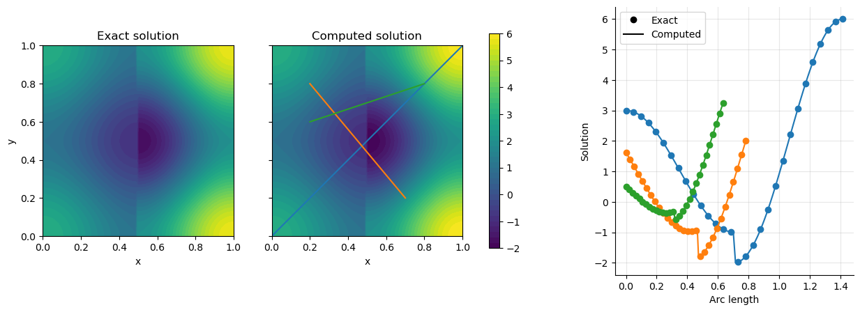
Comparison with exact solution#

The computed and exact solutions agree very well: