Diffusion through a semi-infinite slab#
This verification case from TMAP7’s V&V report [3] consists of a semi-infinite slab with no traps under a constant concentration \(C_0\) boundary condition on the left.
FESTIM Code#
Show code cell content
import festim as F
import numpy as np
import sympy as sp
from scipy.special import erf
from matplotlib import pyplot as plt

C_0 = 1 # atom m^-3
D = 1 # m^2 s^-1
profile_time = 25 # s
exact_solution = lambda x, t: C_0 * (1 - erf(x / np.sqrt(4*D*t)))

model = F.Simulation()

### Mesh Settings ###
vertices = np.concatenate([
    np.linspace(0, 1, 100),
    np.linspace(1, 20, 200),
])

model.mesh = F.MeshFromVertices(vertices)

model.boundary_conditions = [
    F.DirichletBC(surfaces=[1], value=C_0, field="solute")
]

model.materials = [F.Material(id=1, D_0=D, E_D=0)]

model.T = F.Temperature(500)  # ignored in this problem

model.dt = F.Stepsize(
    initial_value=0.01,
    stepsize_change_ratio=1.1,
    milestones=[profile_time]
)

model.settings = F.Settings(
    absolute_tolerance=1e-10,
    relative_tolerance=1e-10,
    final_time=30
)

test_point_x = 0.45
derived_quantities = F.DerivedQuantities(
    [F.PointValue("solute", x=test_point_x)]
)
model.exports = [
    derived_quantities,
    F.TXTExport(
        field="solute",
        filename="./tmap_1b_concentration.txt",
        times=[profile_time]
    ),
]

model.initialise()
model.run()
Defining initial values
Defining variational problem
Defining source terms
Defining boundary conditions
Time stepping...
Calling FFC just-in-time (JIT) compiler, this may take some time.
Calling FFC just-in-time (JIT) compiler, this may take some time.
0.0 %        1.0e-02 s    Elapsed time so far: 1.5 s
0.1 %        2.1e-02 s    Elapsed time so far: 1.5 s
0.1 %        3.3e-02 s    Elapsed time so far: 1.5 s
0.1 %        4.6e-02 s    Elapsed time so far: 1.5 s
0.2 %        6.1e-02 s    Elapsed time so far: 1.5 s
0.3 %        7.7e-02 s    Elapsed time so far: 1.5 s
0.3 %        9.5e-02 s    Elapsed time so far: 1.5 s
0.4 %        1.1e-01 s    Elapsed time so far: 1.5 s
0.5 %        1.4e-01 s    Elapsed time so far: 1.5 s
0.5 %        1.6e-01 s    Elapsed time so far: 1.5 s
0.6 %        1.9e-01 s    Elapsed time so far: 1.5 s
0.7 %        2.1e-01 s    Elapsed time so far: 1.5 s
0.8 %        2.5e-01 s    Elapsed time so far: 1.5 s
0.9 %        2.8e-01 s    Elapsed time so far: 1.5 s
1.1 %        3.2e-01 s    Elapsed time so far: 1.5 s
1.2 %        3.6e-01 s    Elapsed time so far: 1.5 s
1.4 %        4.1e-01 s    Elapsed time so far: 1.5 s
1.5 %        4.6e-01 s    Elapsed time so far: 1.5 s
1.7 %        5.1e-01 s    Elapsed time so far: 1.5 s
1.9 %        5.7e-01 s    Elapsed time so far: 1.5 s
2.1 %        6.4e-01 s    Elapsed time so far: 1.5 s
2.4 %        7.1e-01 s    Elapsed time so far: 1.5 s
2.6 %        8.0e-01 s    Elapsed time so far: 1.5 s
3.0 %        8.8e-01 s    Elapsed time so far: 1.5 s
3.3 %        9.8e-01 s    Elapsed time so far: 1.5 s
3.6 %        1.1e+00 s    Elapsed time so far: 1.5 s
4.0 %        1.2e+00 s    Elapsed time so far: 1.5 s
4.5 %        1.3e+00 s    Elapsed time so far: 1.5 s
5.0 %        1.5e+00 s    Elapsed time so far: 1.5 s
5.5 %        1.6e+00 s    Elapsed time so far: 1.6 s
6.1 %        1.8e+00 s    Elapsed time so far: 1.6 s
6.7 %        2.0e+00 s    Elapsed time so far: 1.6 s
7.4 %        2.2e+00 s    Elapsed time so far: 1.6 s
8.2 %        2.5e+00 s    Elapsed time so far: 1.6 s
9.0 %        2.7e+00 s    Elapsed time so far: 1.6 s
10.0 %        3.0e+00 s    Elapsed time so far: 1.6 s
11.0 %        3.3e+00 s    Elapsed time so far: 1.6 s
12.1 %        3.6e+00 s    Elapsed time so far: 1.6 s
13.4 %        4.0e+00 s    Elapsed time so far: 1.6 s
14.8 %        4.4e+00 s    Elapsed time so far: 1.6 s
16.3 %        4.9e+00 s    Elapsed time so far: 1.6 s
17.9 %        5.4e+00 s    Elapsed time so far: 1.6 s
19.8 %        5.9e+00 s    Elapsed time so far: 1.6 s
21.8 %        6.5e+00 s    Elapsed time so far: 1.6 s
24.0 %        7.2e+00 s    Elapsed time so far: 1.6 s
26.4 %        7.9e+00 s    Elapsed time so far: 1.6 s
29.1 %        8.7e+00 s    Elapsed time so far: 1.6 s
32.0 %        9.6e+00 s    Elapsed time so far: 1.6 s
35.2 %        1.1e+01 s    Elapsed time so far: 1.6 s
38.8 %        1.2e+01 s    Elapsed time so far: 1.6 s
42.7 %        1.3e+01 s    Elapsed time so far: 1.6 s
47.0 %        1.4e+01 s    Elapsed time so far: 1.6 s
51.8 %        1.6e+01 s    Elapsed time so far: 1.6 s
57.0 %        1.7e+01 s    Elapsed time so far: 1.6 s
62.7 %        1.9e+01 s    Elapsed time so far: 1.6 s
69.0 %        2.1e+01 s    Elapsed time so far: 1.6 s
75.9 %        2.3e+01 s    Elapsed time so far: 1.6 s
83.3 %        2.5e+01 s    Elapsed time so far: 1.6 s
Calling FFC just-in-time (JIT) compiler, this may take some time.
91.5 %        2.7e+01 s    Elapsed time so far: 2.4 s
100.0 %        3.0e+01 s    Elapsed time so far: 2.4 s
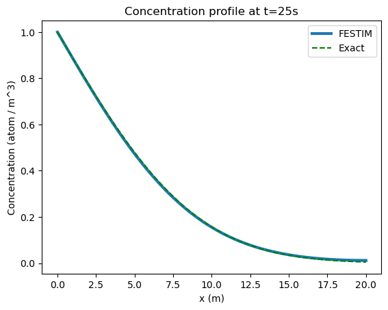
Comparison with exact solution#
The exact solution is given by
\[
c(x, t) = c_0 \left( 1 - \mathrm{erf}\left( \frac{x}{2\sqrt{Dt}} \right) \right)
\]
Show code cell source
# plotting computed data
computed_data = np.genfromtxt("./tmap_1b_concentration.txt", delimiter=",", skip_header=1)
computed_x = computed_data[:, 0]
computed_solution = computed_data[:, 1]
plt.plot(computed_x, computed_solution, label="FESTIM", linewidth = 3)

# plotting exact solution
exact_y = exact_solution(np.array(computed_x), profile_time)
plt.plot(computed_x, exact_y, label="Exact", color="green", linestyle="--")

plt.title(f"Concentration profile at t={profile_time}s")
plt.ylabel("Concentration (atom / m^3)")
plt.xlabel("x (m)")

plt.legend()
plt.show()
Show code cell source
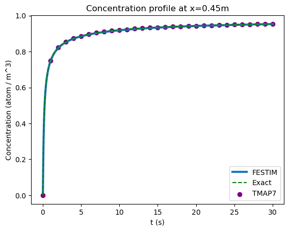
# plotting computed data
computed_solution = derived_quantities[0].data
t = derived_quantities[0].t
plt.plot(t, computed_solution, label="FESTIM", linewidth = 3)

# plotting exact solution
exact_y = exact_solution(test_point_x, np.array(t))

plt.plot(t, exact_y, label="Exact", color="green", linestyle="--")

# plotting TMAP data
tmap_data = np.genfromtxt("./tmap_point_data.txt", delimiter=" ", names=True)
tmap_t = tmap_data["t"]
tmap_solution = tmap_data["tmap"]
plt.scatter(tmap_t, tmap_solution, label="TMAP7", color="purple")

plt.title(f"Concentration profile at x={test_point_x}m")
plt.ylabel("Concentration (atom / m^3)")
plt.xlabel("t (s)")

plt.legend()
plt.show()